The app is an open educational resource funded through the SimBiose project by the Digital Teaching Fund at TU Dresden.
You may freely use the app as a whole as well as individual components in accordance with the Creative Commons license CC BY-SA 4.0 (share, edit, attribution, redistribute under the same terms). If you remix, modify, or otherwise build directly upon the material, you may distribute your contributions only under the same license as the original.
No warranty is provided for the accuracy of the content or the technical functionality.
Developer source code
https://github.com/tpetzoldt/simbiose-w


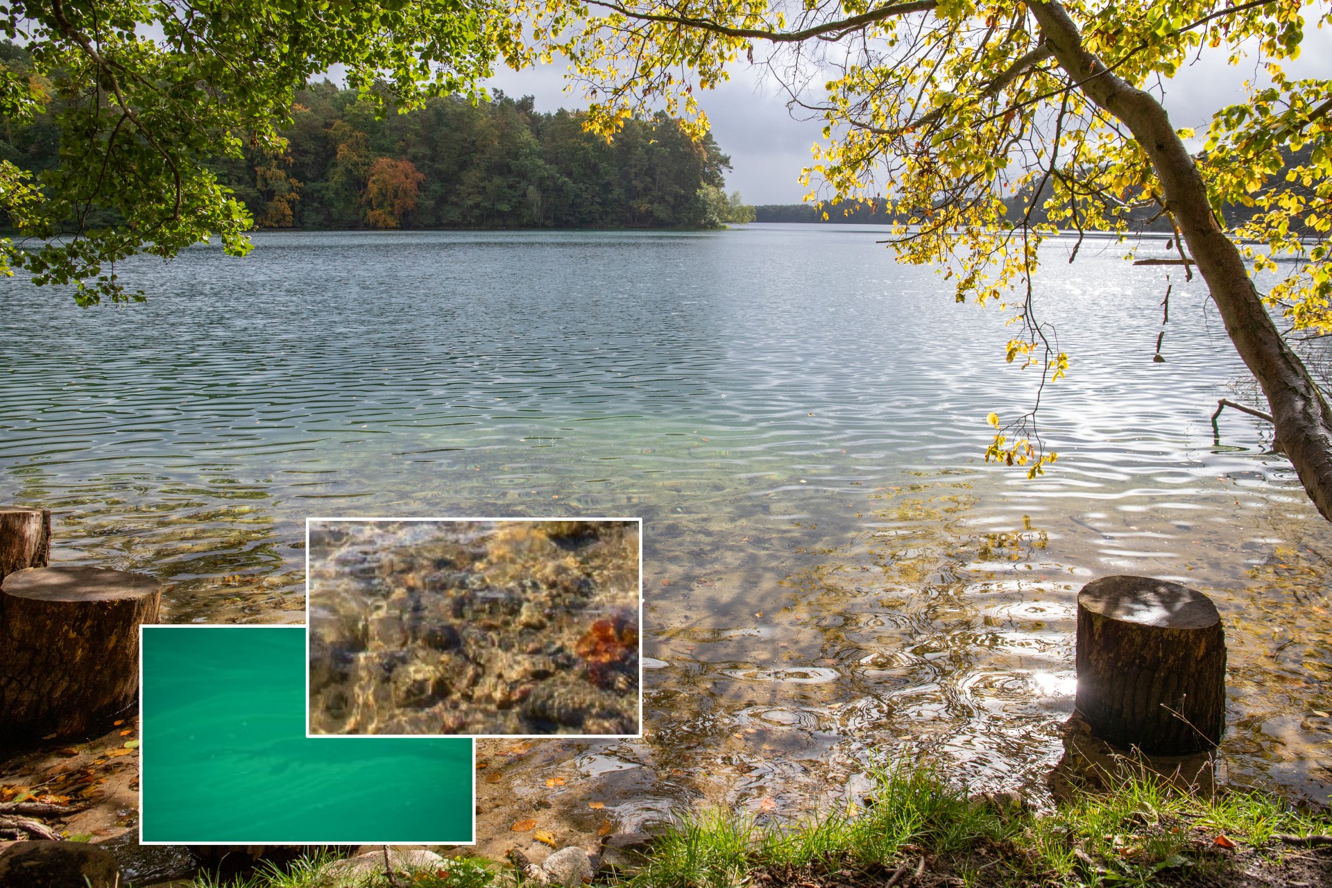 photo: Felix Grunicke
When we look into a swimming lake from the shore, the water is sometimes so clear that we can see to the bottom. If we look closely, we might even spot some animals, such as daphnia (water fleas).
Anyone who often walks along the shore can observe that a lake might not always be clear. Sometimes it is turbid from microscopic algae (phytoplankton) and turns green. Phytoplankton is very important for the food chain, because it feeds the zooplankton, which in turn feeds the fish. On the other hand, heavy phytoplankton blooms can lead to serious problems. Swimming in the lake is then prohibited. When extracting drinking water from reservoirs, the algae must be removed at the water treatment plant.
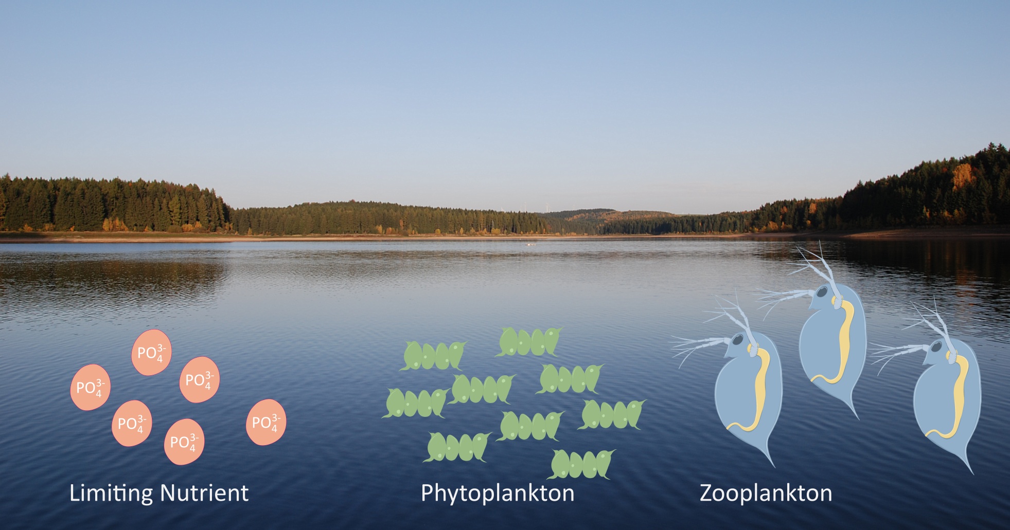 photo: tpetzoldt
The shift from clear to green, turbid water results from fluctuations in population density. This can happen quickly because microalgae and daphnia grow and reproduce very rapidly. In nature, the rate of growth depends on many factors, such as the season, the weather, nutrient availability, and fish stock.
Scientists around the world are working to better understand these processes and describe them mathematically in order to understand the condition of water bodies and, for example, predict algal blooms. To do this, they use mathematical models and, more recently, machine learning. In addition, a great amount of data must be collected.
The exact timeline of algal growth is difficult to predict in reality because many different species of phytoplankton and zooplankton are present in a lake, and many environmental factors act simultaneously. Nevertheless, the example of “algal growth in a lake” can help us understand basic growth processes. Growth can be found everywhere in nature – in plants, insects, and wildlife. Similar models are also used to model the spread of diseases, for example during the COVID-19 pandemic.
In the “Population Growth” app, we will explore some fundamental growth processes. We will start with an unlimited, exponential growth model, then examine forms of limited growth, and finally look at a predator-prey interaction between two populations.
The app is optimized for display on laptop and PC monitors and on popular tablets.
If the text is still too large or too small, you can adjust the font size in your system settings or web browser:
- Windows: [Ctrl] + [-] or [Ctrl] + [+]
- Android/Chrome: Settings – Accessibility
- iPad: if text overlaps, close all other tabs
Portrait mode is supported on smartphones.
Development team at TU DresdenThomas Petzoldt, Luisa Henze, Monique Meier
Technologies

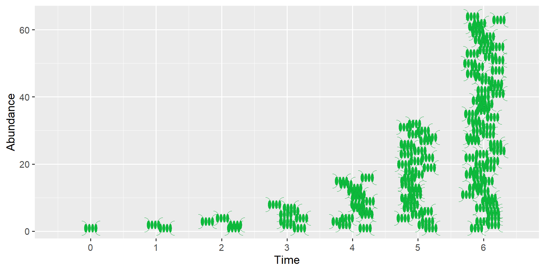
Single-celled organisms, such as bacteria or phytoplankton, can reproduce very quickly. The figure shows schematically how the number of phytoplankton cells doubles with each division. This results in a geometric sequence: 1-2-4-8-16-32-64, and so on.
To describe such a growth process, three basic pieces of information are needed:
The number of organisms present. This is called abundance and is usually denoted by the symbol \(N\) (number).
The population growth per unit of time, in this case doubling.
The underlying time interval \(\Delta t\) during which the growth occurs, e.g., a day, an hour, or a year.
The greater the existing abundance, the greater the increase. One cell becomes two; 8 cells become 16.
The greater the increase, the faster the population grows. Instead of doubling (factor = 2, growth = 100%), the organisms could also increase tenfold (factor = 10, growth = 900%), but only a small portion may reproduce, e.g., growth = 10%, in which case the factor = 1.1.
The smaller the time step in which reproduction occurs, the faster the population growth.
Discrete Growth
In discrete growth, cell division occurs at fixed time intervals.
The number of cells (the abundance \(N\)) at a future time \(t+1\) is the abundance of cells at the current time \(t\) plus the number of new cells added \(b\cdot N_{t}\). Here, \(b\) is the per-capita reproduction rate (birth rate), the proportion of cells that divide.
\[ N_{t+1} = N_{t} + b \cdot N_{t} \]The abundance \(N\) is either dimensionless and means “number of individuals,” but it can also be specified with a unit of measurement, e.g., individuals per square meter or per liter. A concentration value is also possible, e.g., mg/L biomass or mg/L carbon.
Instead of the birth rate \(b\), the symbol \(r\) is often used, representing the net reproduction rate. This consists of two parts: the birth rate \(b\) and the death rate \(d\). Depending on whether the difference \(r=b-d\) is positive or negative, the population grows or declines.
A birth rate \(r=1\) means that for every existing individual, a new individual is added per time step, resulting in a doubling of the population.
Continuous GrowthWhen considering a very large number of individuals that reproduce continuously—that is, not at fixed intervals—we refer to this as exponential growth. The equation above becomes an exponential function:
\[ N_t = N_0 \cdot e^{r \cdot t} \]This function describes the development of the number of individuals (abundance, \(N\)) at time \(t\) as a function of the net reproduction rate \(r\) and the initial abundance \(N_0\) at time \(t=0\).
For animals that reproduce only once a year, discrete growth models are typically used in practice, while continuous models are typically used for microorganisms.
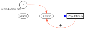
The System DiagramA so-called system diagram can be used for illustration purposes:
- In this diagram, a thick-bordered rectangle represents a state variable, e.g., the abundance of a population,
- thick arrows represent a flow of matter or energy, and
- thin arrows represent an interaction.
- Metabolic processes, e.g., growth, are symbolized by a hexagon in this example,
- while fixed parameters, metabolic rates, and auxiliary variables are represented by circles.
Positive (enhancing) feedback can be symbolized by a (+), and negative feedback by a (-).
- Given a growth rate of \(r=1\) d-1, how many cells will develop from a single cell in one day:
- in discrete growth at fixed time intervals?
- with continuous (exponential) growth?
- A green algae population starts with 10 cells per liter and a growth rate of \(r=1\) d-1. How many cells per liter will there be after 7 days of exponential growth?
- A cyanobacteria population (blue-green algae) grows at a rate of \(r=0.5\) d-1. After approximately how many days will the abundance have increased tenfold under exponential growth?
- A clear-water situation has developed in a lake. The Daphnia population, with a concentration of 50 individuals per liter, is suffering from acute food shortage and is no longer reproducing. However, due to predation by fish, the exponential mortality rate is \(d=0.1\) d-1. After how many days will there be only one Daphnia left in one liter of water?
- A thought experiment: A beaker containing 1 L of nutrient solution holds algae with a fresh mass of 1 mg L-1, and the growth rate is 1 d-1. How long would it take until the beaker is completely filled with algal biomass if the algae could grow without limitation?
- If the numbers get too large, you can shorten the simulation period.
- You can read the numbers directly from the graph using the mouse pointer.
- You can save the results graph by clicking the camera icon.
- Instead of a simulation, a pen and paper or a calculator can sometimes be useful—and thinking things through is always a good idea.
- If a population is dying off, i.e., \(b < d\), then the reproduction rate \(r\) is negative.
- The density of algae is only slightly greater than that of water. We can practically assume a density of 1 g cm-3.
The introduction assumed a doubling rate, but for continuous growth, an exponential function is used. Why an exponential function and not a power law??
In reality, not all algae cells divide at the same time. Some divide earlier, others later, and the ones that divide earlier may already be dividing for the second time. As a result, we do not obtain a geometric sequence, but rather exponential growth.
From the step-by-step (iterative) equation:
\[ N_{t+1} = N_{t} + r \cdot N_{t} \] we obtain, by rearranging, a difference equation:
\[ \frac{N_{t+1} - N_t}{\Delta t} = r \cdot N_t \] or:
\[ \frac{\Delta N}{\Delta t} = r \cdot N_t \]If we consider a very large number of cells and short time intervals, we obtain a differential equation:
\[ \frac{dN}{dt} = r \cdot N \]This equation can be analytically integrated using the so-called variable separation method to yield the exponential formula:
\[ N_t = N_0 \cdot e^{r\cdot t} \]The exponential formula has the advantage that one does not have to iterate step by step, but can calculate the values for all time steps directly.
Initial Values
Parameters
Control
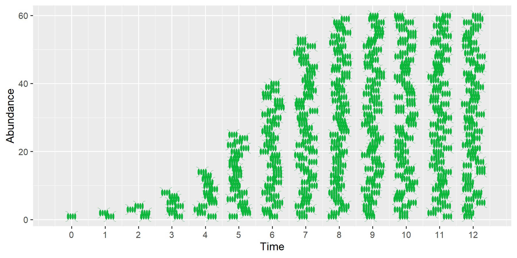
Simulations of exponential growth clearly show that unlimited growth can lead to an unimaginably large population size after a relatively short time.
Let’s assume we have a single water flea with a length of 1.5 mm and a mass of 0.25 mg, with a population growth rate of \(r=0.1\) per day (d-1). With unlimited reproduction, after 6 months we would already have 80 million daphnia with a total mass of 20 kg. After 14 months, Lake Müritz, Germany’s largest lake with a volume of 737 million m^3, would be completely filled with Daphnia. In just over 15 months, even Lake Constance would be.
In reality, population growth slows as abundance increases, resulting in an S-shaped growth curve. One of the simplest models for this is so-called “logistic growth.”
The logistic model is one of the most important formulas in population ecology. However, it does not account for what causes the limitation. In daphnia, this can be caused by food scarcity or oxygen deficiency. In algae, self-shading occurs because the algae cells block light from one another. Some microorganisms possess the ability to self-regulate. They can detect cell density through chemical secretions from other cells and divide less frequently before light and nutrients become scarce.
Limits of Growth
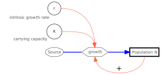
In logistic growth, the growth rate \(r\) is no longer constant but is a function of abundance:
\[ r = r_{max} \cdot \left(1 - \frac{N}{K}\right) \]Here, the actual growth rate \(r\) is given by the product of the species-specific (intrinsic) reproduction rate \(r_{max}\) and a dimensionless term \(\left(1 - \frac{N}{K}\right)\), where \(r\) is the realized reproduction rate and \(K\) is the carrying capacity.
The growth equation can then be written as:
\[ N_t = \frac{K N_0 e^{r t}}{K + N_0 (e^{r t}-1)} \]This looks quite complicated, but it is easy to calculate. In reality, this formula is the solution to a differential equation:
\[ \begin{align} \frac{dN}{dt} &= r_{max} \cdot \left(1 - \frac{N}{K}\right) \cdot N \end{align} \]This equation describes the change in population per unit of time, exactly as shown in the system diagram.
ExplanationGrowth continues until the carrying capacity \(K\) is reached. At low population density, i.e., when \(N \ll K\), the term in parentheses is approximately equal to 1 and growth is at its maximum. The product \(r \cdot \left(1 - \frac{N}{K}\right)\) is approximately \(r\).
The closer the abundance \(N\) approaches the carrying capacity, the smaller \(r \cdot \left(1 - \frac{N}{K}\right)\) becomes, converging to zero as \(N \rightarrow K\).
Set the logistic growth rate to the smallest possible value (\(r_{max}=0.02\)) and the carrying capacity \(K=500\):
- What shape does the growth curve take?
Now adjust the \(K\) slider.
Why does increasing \(K\) have only a minor effect?
Why does decreasing \(K\) have a greater effect?
Now set \(r_{max}=0.1\) and \(K=100\) again.
What happens if you change the initial abundance \(N_0\)?
Now set the initial abundance to a larger value, e.g., 120. What happens?
In the following, we will examine different types of equilibrium:
- \(N_0=0, r_{max}=0.1, K=100\)
- \(N_0=1, r_{max}=0, K=100\)
- \(N_0=100, r_{max}=0.1, K=100\)
First, explain by interpretation how the different equilibrium states arise.
Try to understand why equilibrium is reached by substituting the values into the equations. For this, the derivative equation \(dN/dt= ...\) is easier to understand than the integral form.
When the initial abundance \(N_0\) is small compared to \(K\), the growth curve initially approaches exponential growth. The abundance is far from \(K\), so its increase no longer has any effect.
When \(K\) is reduced to a value close to the abundance, the limitation becomes clearly visible and the growth curve flattens out.
The value of \(N_0\) only influences how quickly the value of \(K\) is reached. It has no influence on the final value.
If the initial abundance exceeds the carrying capacity, the population decreases until \(K\) is reached.
In the experiment, we can identify three different types of equilibria. If \(N_0=0\), there are no organisms present that can grow. We have, so to speak, a “sterile system.” The abundance remains at 0.
If \(r_{max}=0\) and \(N_0 > 0\), then organisms are present, but they do not reproduce. It is also possible that they reproduce, but reproduction and death are exactly balanced.
Both equilibria are “labile” (or unstable). If even a small value is added to \(N_0 = 0\), population growth begins, the equilibrium is left, and the abundance moves toward \(K\). The same phenomenon can be observed in the second case when \(r_{max} > 0\).
In the third case (at \(N = K\)), the equilibrium is stable. It is reached when \(N\) is less than \(K\) but also when \(N\) is greater than \(K\). Even if the abundance temporarily deviates from \(K\), its value us quickly restored. This is called “resilience.”
The logistic model provides the theoretical basis for distinguishing between so-called r- and K-strategists. An r-strategist refers to species that reproduce rapidly, “at any cost”. K-strategists, on the other hand, are species that can achieve a high abundance (a high K). According to a more modern interpretation, these are organisms that can survive well and minimize losses even during resource shortages.
See also r/K selection theory on Wikipedia.
Discrete growth can lead to chaosThe logistic model and its equilibria are a textbook example from chaos theory. The experiments described under “Exercises” assume that population growth occurs continuously, i.e., can be described mathematically by a differential equation.
If population growth occurs in the form of generations, e.g., in wild animals that reproduce only once a year, then the time step is “discrete”. Mathematically, this is a difference equation.
In this case, the carrying capacity may be temporarily exceeded. This is then followed by a partial collapse of the population, e.g., due to a lack of food. In the following time step, the population can recover again, and so on. This creates a cycle and, under certain conditions, a chaotic pattern.
More information on this can be found under [Logistic Map]https://en.wikipedia.org/wiki/Logistic_map#Discretization_of_the_logistic_equation) on Wikipedia.
If you want to try it out yourself, you can send an email to the app’s developers. Perhaps they will then incorporate the chaos model into the app.
Initial Values
Parameters
The logistic growth model is of high theoretical importance and is frequently used in practice, for example in laboratory growth experiments with bacteria and algae or in the industrial biotechnological production of pharmaceuticals.
However, the logistic model has two major drawbacks:
One must specify beforehand where the capacity limit \(K\) lies, e.g., from a previous experiment.
It is not known why growth stops – whether, for example, a nutrient has been depleted or whether the algae are shading each other too much.
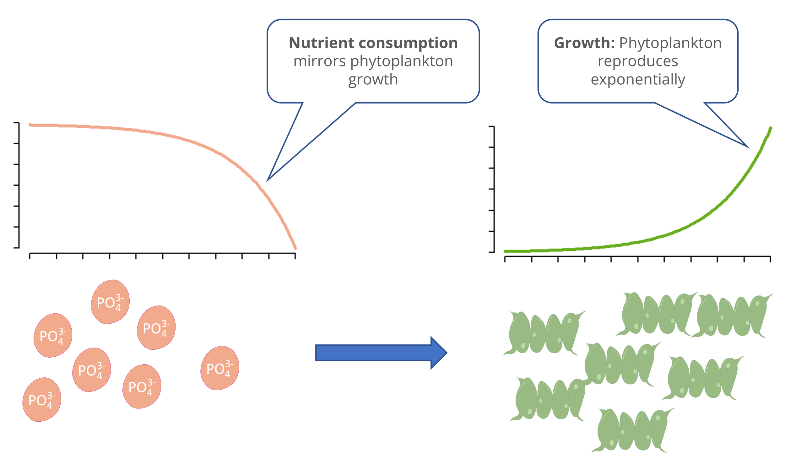
In the resource-limited growth model, this problem is solved by specifying an additional equation for a limiting resource. As the phytoplankton grows, a resource is consumed, e.g., phosphorus. When the phosphorus is depleted, growth stops. The curves for phytoplankton and phosphorus exhibit mirroring behavior.
Instead of phosphorus, nitrogen can also be the limiting factor, or both. In that case, an additional equation is required (multiple limitation). The influence of light and temperature can also be taken into account.
Phosphorus Limitation of Algal Growth
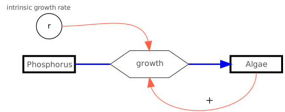
In this example, we will describe the population growth of phytoplankton as a function of phosphorus (\(P\) in mg m^-3). To avoid duplicate letters, we will refer to the phytoplankton as “algae” \(A\). As a unit of measurement, we will use the biovolume or the carbon contained in the organisms in mg m-3. For time, we will use measurement hours (h).
\[ \begin{align} \frac{dA}{dt} &= r(P) \cdot A \\ \frac{dP}{dt} &= - r(P) \cdot A \cdot \frac{1}{Y}\\ r(P) &= r_{max} \cdot \frac{P}{k_P + P} \end{align} \]In more modern models, biomass is often expressed in units of carbon. Carbon is the “element of life” and accounts for approximately 50% of the dry weight in most organisms.
The first equation \(dA/dt\) is, in principle, the exponential growth equation again; however, the growth rate \(r\) is now a function of \(P\), i.e., \(r=f(P)\). When the nutrient \(P\) is depleted, the growth rate \(r(P)\) approaches zero.
The first part of the phosphorus equation \(dP/dt\) corresponds to the algae equation, but with a negative sign. When algae grow, phosphorus is consumed. The conversion factor \(1/Y\) is used to convert the phosphorus and carbon content of the algae stoichiometrically. Here, one typically uses the reciprocal of the yield coefficient \(Y\) (“Yield”). A value of \(Y=41\) means that for every 1 mg of phosphorus, 41 mg of carbon is bound in the biomass.
The function \(r(P)\) describes the dependence of the growth rate \(r\) on phosphorus as so-called saturation kinetics. As the phosphorus concentration increases, the growth rate initially rises steeply. When there is a nutrient surplus, the curve flattens out and approaches a maximum value \(r_{max}\). The value \(k_P\) is the nutrient concentration at which 50% of the maximum growth rate is reached. The smaller \(k_P\) is, the better an algal species is adapted to low nutrient concentrations.
Compare resource-limited growth with logistic growth.
What is the advantage of resource-limited growth over the logistic growth function?
Are there any disadvantages?
Examine the influence of \(r\), \(k_P\), and \(Y\) on growth.
At what values of \(r\) is growth fastest?
At what values of \(k_P\) is growth fastest and nutrient utilization best?
What determines the steepness of the transition to the limiting phase?
Which parameter and which initial value determine the maximum phytoplankton abundance reached? This value corresponds to the carrying capacity \(K\) in the logistic model.
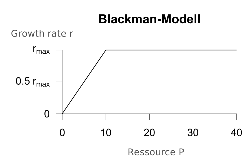
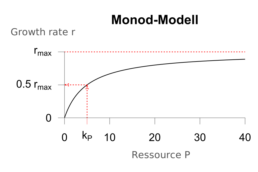
The relationship between the growth rate \(r\) and the nutrient concentration is described by what is known as kinetics. This refers to how fast the algae grow; this is also called a functional response. In contrast, the actual growth models (e.g., the logistic and resource-limited models) describe how many algae can grow in total. This is called a numerical response.
For the dependence of the growth rate on a resource (e.g., phosphorus), saturation kinetics are used. The more nutrients are available, the faster the growth. Above a certain nutrient concentration, saturation is reached, meaning that even more nutrients do not lead to further growth.
There are various ways to describe this mathematically. In the Blackman model, the growth rate initially increases proportionally with the nutrient concentration. Here, \(k_b\) is the proportionality factor. When the nutrient concentration (\(P\)) exceeds the maximum possible growth rate (\(r_{max}\)), the growth rate \(r\) remains constant at \(r_{max}\):
\[ r = r_{max} \cdot \min(k_b \cdot P, 1) \] The Monod model assumes a gradual transition from the growth phase to saturation. In the equation used for this purpose:
\[ r = r_{max} \cdot \frac{P}{k_P + P} \]the limitation is achieved through a ratio in which the denominator is a so-called half-saturation rate \(k_P\), which has the same unit of measurement as \(P\). This makes this term dimensionless. If the phosphorus concentration and the half-saturation rate are equal (i.e., \(P=k_P\)), then the ratio \(P/(P + P) = 0.5\). However, if \(P\) is very large (\(P >> k_P\)), then the ratio converges to 1 and the growth rate \(r\) converges to \(r_{max}\).
Fast-growing phytoplankton species have a high maximum growth rate, while species that can survive on few nutrients have a low semi-saturation constant.
The use of fertilizers in agriculture is very important for our food supply, but it is crucial to avoid overfertilization. Excess phosphorus and nitrogen cannot be absorbed by plants and ends up in our rivers and lakes, and ultimately in the sea.
In these bodies of water, increased phosphorus and nitrogen inputs lead to increased phytoplankton growth, and the water becomes turbid. In deep water, the decay of algae then leads to oxygen depletion. The increased growth of plankton and aquatic plants and the resulting deterioration of water quality is called eutrophication.
Further information on nutrient input and eutrophication can be found, for example, on the website of the German Federal Environment Agency.
Initial Values
Parameters
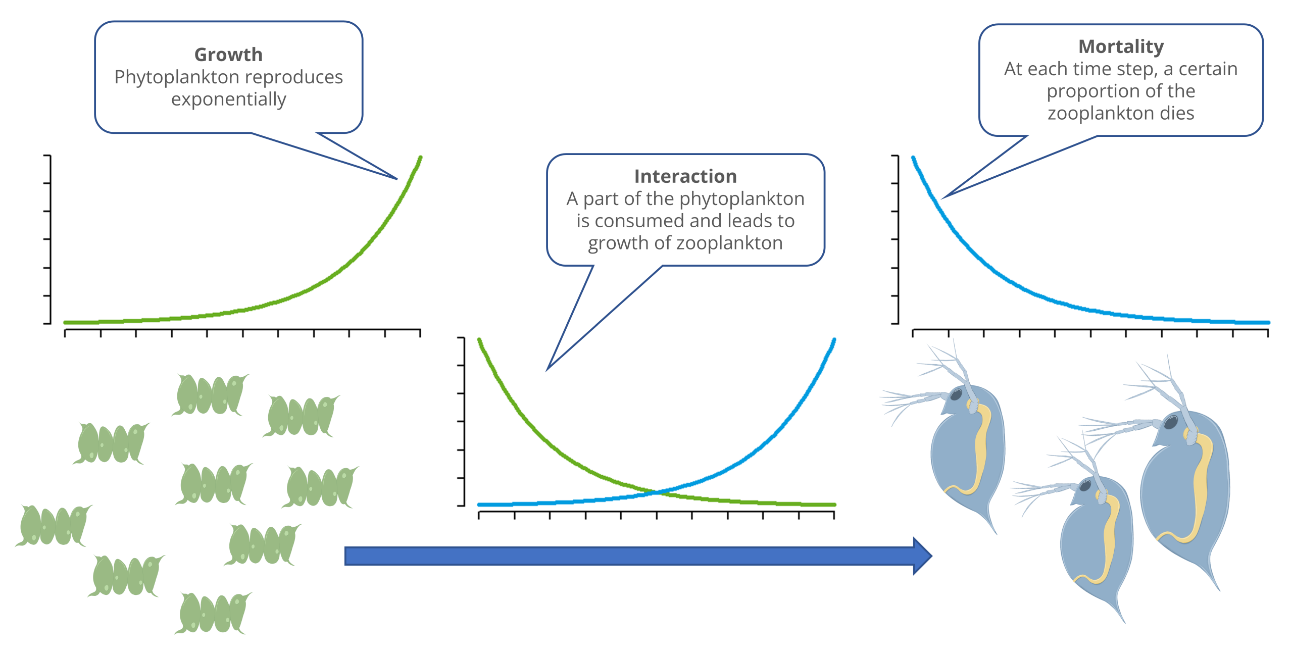
The models considered so far each describe only the growth of a single population. In reality, multiple populations are almost always found together, either competing with one another or forming food chains and food webs.
In the following, we will examine a segment of a food chain involving a prey population and a predator population, e.g., phytoplankton (algae) and zooplankton (daphnia).
The Predator-Prey Model of Lotka and Volterra
Unlike in logistic or resource-limited growth, stable equilibria are rarely observed in nature; instead, population abundance fluctuates. There are various reasons for this, such as the reproductive cycle or variations in food availability due to the seasons and weather.
However, population fluctuations can also result from interactions between populations.
Such interactions were investigated and mathematically described in the early 20th century by the Italian mathematician and physicist Vito Volterra and the Austrian-American chemist and actuary Alfred Lotka.
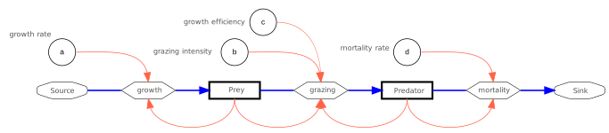
Their model consists of two equations, one for the prey population (e.g., algae) and one for the predator population (e.g., daphnia). As a modification to the notation of the equations originally used by Volterra (1926), many scientists and textbooks use different symbols and variants. In the following, we use a simplified notation with \(B\) for the prey population and \(R\) for the predator population. For the model parameters, we use consecutive letters \(a, b, c, d\), which can be interpreted as follows:
\(a\): Reproduction rate of phytoplankton (prey population)
\(b\): Loss of phytoplankton (prey) due to predation by daphnia (predators)
\(c\): Growth efficiency of daphnia (predators) due to food intake
\(d\): Mortality rate of daphnia (predators)
The model essentially consists of three processes. The growth of the prey population (e.g., algae) and the decline of the predator population (e.g., Daphnia) each correspond to an exponential growth model with a positive or negative rate of change, respectively.
Exponential growth of the prey population:
\[ \frac{dB}{dt} = a \cdot B\\ \]Exponentielles Absterben der Räuberpopulation:
\[ \frac{dR}{dt} = - d \cdot R\\ \]The third process describes the interaction between predators and prey. Here, the rate of decline in the prey population \((b \cdot R)\) depends on the abundance of the predator population, and the growth rate of the predator population depends on the abundance of the prey population \((c \cdot B)\). By choosing different values for \(b\) and \(c\), one can account for trophic efficiency (\(c/b\)), e.g., that only 10% of the food is used for reproduction.
This results in the following system of equations, in which, for clarity, the loss rate of the prey population due to predation and the growth rate of the predator population are denoted by additional parentheses:
System of Equations \[ \begin{align} \frac{dB}{dt} &= a \cdot B - (b \cdot R) \cdot B \\ \frac{dR}{dt} &= (c \cdot B) \cdot R - d \cdot R \end{align} \]The parentheses are for illustrative purposes only and are usually omitted.
The initial standard parameters and starting values are as follows:
\(a=b=c=d=0.1\), \(B_0=1\), \(R_0=0.5\).
- Change the initial value for the predator (\(R_0\)) to 2 or 1.
- What happens?
- Set \(R_0=2\) again. Now try to find a prey reproduction rate (\(a\)) at which an equilibrium is reached again.
- You can find the desired value either by trial and error or by rearranging the system of equations.
Period and Amplitude
First, restore the default parameters, e.g., by reloading the app.
By changing the parameters \(a, b, c, d\), you can alter the period. For simplicity, let all parameter values be equal at first (\(a = b = c = d\)). Now find values such that the period:
- shortens
- lengthens
Why do the parameters affect the period in the observed direction?
Note: Checking the “Scan values” box activates additional guide lines. You can read specific values using the mouse.
Now set the parameter values back to their defaults.
Double the prey reproduction rate \(a\) to 0.2. How can the result be explained?
Double the predator mortality rate \(d\) to 0.2. How can the result be explained?
What conclusions can be drawn regarding turnover and population density in real-world systems?
- Double and halve the turnover between \(B\) and \(R\). Use parameters in the range: \(b = c = 0.05 \dots 0.2\).
- How can the result be explained? What information is needed to assess whether the result is realistic?
Analytical Determination of Equilibrium and Mean Values
Rearrange the system of equations and determine the equilibrium state.
At equilibrium, the first derivatives of both equations are equal to 0. Return to Problem (2) and find the value of the parameter a by rearranging and solving the system of equations.
Using the “Read Values” checkbox, you can estimate the mean values of prey and predator for each cycle from the displayed points. Here, a cycle always extends from one maximum to the next.
Compare the equilibrium state (horizontal dotted lines) with the mean values estimated in (b). Consider or research how the mean value can be obtained directly from the initial values and the model parameters.
We are usually taught that coordinate axes should always be labeled with units of measurement. This is very important, but there are exceptions. In theoretical models, sometimes only the variable name – without a unit of measurement – is written on the axis, e.g., “time,” “frequency,” or “abundance.”
Physicists go even further and scale all axes to an interval from zero to one. In our apps, we have chosen not to do this, so that users can visualize what the values represent. This allows us to specify a unit of measurement depending on the application, e.g., “hours” or “days” for fast-growing algae and Daphnia, or “years” for snowshoe hares and lynx.
When it comes to units of measurement for abundance and biomass, it is important to note that algae and Daphnia vary in size and have different body masses. If we omit the unit of measurement, the values on the y-axis are merely relative quantities that cannot be compared with one another.
When considering biomass, we can use a trick to establish approximately comparable ratios. As a rule of thumb, about 10% of the energy is transferred from one trophic level to the next in a food chain.
We can account for this if we set the parameter \(c\) (“growth efficiency”) to one-tenth of \(b\) (“feeding intensity”), i.e., for example, \(b=0.2\) and \(c=0.02\). In this case, the initial values must also be adjusted accordingly, e.g., \(B_0=1\) and \(R_0=0.05\).
By changing the parameters, combinations can also be set that appear nonsensical or unrealistic. This is partly because the parameter values are specified relative to time, e.g., growth per day or per hour. Therefore, it is sometimes necessary to adjust the time unit as well and subject the values and units of measurement to a thorough reality check.
To make the results of the app easier to understand, we can disregard the units of measurement and consider the results only qualitatively, i.e., small-large, cycle–equilibrium, larger amplitude–smaller amplitude, longer cycle–shorter cycle.
The example of snowshoe hares and lynx is often cited in connection with the predator-prey model. Both species live in North America, primarily in Canada.
It has been observed that hunters’ fur sales fluctuate in a cycle of 9 to 11 years. It seemed likely that this was a Lotka–Volterra cycle. Upon closer examination, however, inconsistencies became apparent, and various other explanations were proposed. One explanation was that the fluctuating fur sales were due to the influence of hunters. Another explanation is that the predator-prey cycle results from interactions at a lower trophic level—that is, not as an interaction between snowshoe hares and lynx, but between vegetation and the snowshoe hares. The lynx merely follows the cycle. More details can be found in the Wikipedia article Lotka–Volterra equations.
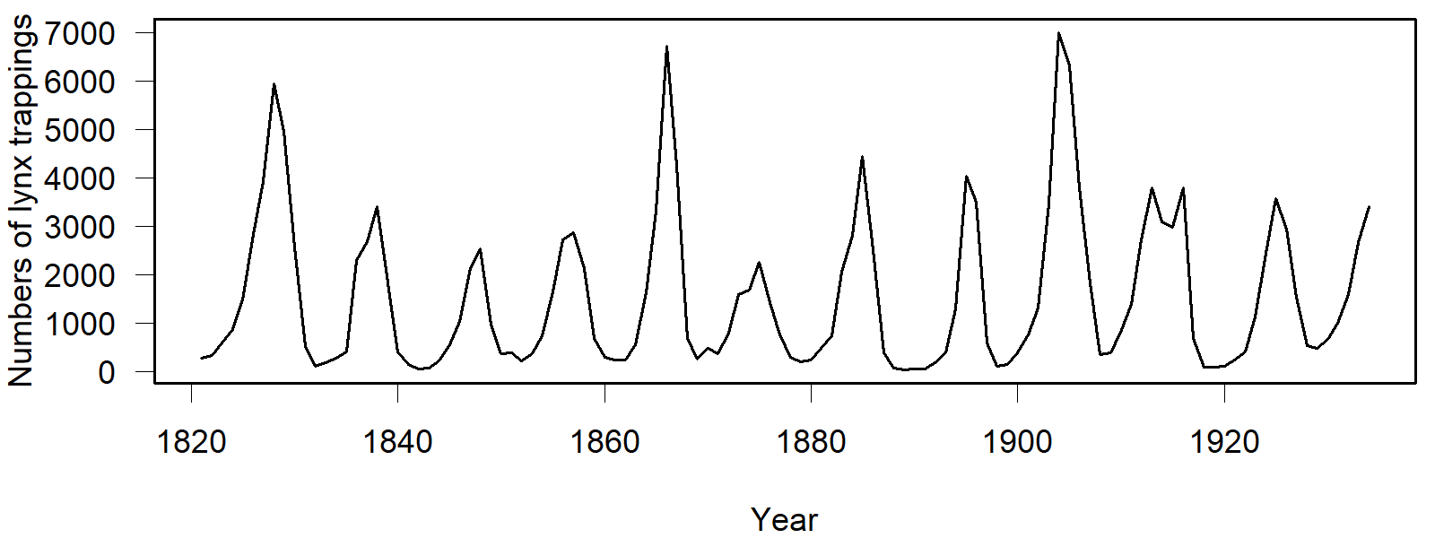 Historical dataset of lynx catches in Canada, from Brockwell & Davis (1991)
The algae-Daphnia system is also used as a textbook example in theoretical ecology. In real water bodies, however, only short section of these dynamics can be observed. An annual spring peak in algae is immediately followed by a distinct clear-water phase. The continuation of these oscillations is then prevented by damping mechanisms such as resource limitations (particularly phosphorus) and integration into a more complex food web (Sommer et al., 2012).
Moose and WolvesAnother prominent example is the interrelationship between moose and wolves. Research on this topic was conducted in the Isle Royale National Park, an island in one of the Great Lakes in North America. It is the longest-running study of predator-prey systems in the world. With the exception of researchers and summer visitors, no humans live on the island.
Lotka–Volterra-type interactions were indeed observed between the moose and the wolves. However, these occurred only during brief phases of a cycle. In reality, additional factors also come into play here, such as parasites that weaken the moose. Conversely, the wolves were temporarily infected by a viral disease and nearly went extinct.
During a particularly cold winter, wolves were observed traveling a distance of 22 km across the frozen lake to reach the island. This confirmed a long-standing assumption that the wolf population on the island is not completely isolated. Interaction with the mainland is apparently vital for the wolf population’s survival, but due to global warming, such ice bridges no longer form every 3 to 4 years, but only once every 10 years.
More information can be found on the National Park’s website, on the research project’s website (https://isleroyalewolf.org/), and in the book by Vucetich (2024). There are also articles on Wikipedia on this topic. The videos about the project on YouTube are highly recommended, e.g., https://youtu.be/DS-4IsDg7mA. Additional videos can be found by searching for the keywords: wolves isle royale.
The examples show that predator-prey interactions are far more complex in practice than the Lotka-Volterra model. The model is not suitable for making predictions, but, as in the app’s simulation experiments, one can derive fundamental insights into the emergence of population fluctuations or the establishment of equilibria.
In practical models, various model components are combined: exponential growth, logistic growth, multiple resources, and predator-prey interactions. Additionally, the models incorporate current data on nutirients, weather, climate, and human influence.
ReferencesBrockwell, P. J. and Davis, R. A. (1991). Time Series and Forecasting Methods. Second edition. Springer. Series G (p. 557).
Sommer, U., Adrian, R., De Senerpont Domis, L., Elser, J. J., Gaedke, U., Ibelings, B., Jeppesen, E., Lürling, M., Molinero, J. C., Mooij, W. M., van Donk, E., & Winder, M. (2012). Beyond the Plankton Ecology Group (PEG) Model: Mechanisms Driving Plankton Succession. Annual Review of Ecology, Evolution, and Systematics, 43, 429–448. doi:10.1146/annurev-ecolsys-110411-160251
Vucetich, J.A. (2021) Restoring the Balance: What Wolves Tell Us about Our Relationship with Nature. Johns Hopkins University Press.
Privacy policy
We use only cookies that are absolutely necessary exclusively for the provision of the service. The cookies will be set automatically by access of this web page, except if setting cookies is disabled in the browser settings. Data processing takes place on the legal basis of section §6 para.1 lit. f GDPR.
- Name of the cookie: weblab.hydro.tu-dresden.de
- Cookie provider: TU Dresden
- Duration of storage: current browser-session, the cookie will be removed after closing the browser
- Purpose: enables the server to accept user input and to send the results back to the web browser
This means specifically that no so-called tracking cookies are used to record or analyse user movements and the surfing behaviour of users of our site.
ImpressumSee the Impressum of TU Dresden with following changes:
Contact person:
Technische Universität Dresden
Institut für Hydrobiologie
Dr. Thomas Petzoldt
01062 Dresden
Tel.: +49 351 463-34954
E-Mail: thomas.petzoldt@tu-dresden.de


Die App Ist eine “Offene Bildungsresource”. Sie dürfen die App als Ganzes sowie einzelne Bausteine gemäß der Creative Commons Lizenz CC BY-SA 4.0 frei verwenden (teilen, bearbeiten, Namensnennung, Weitergabe unter gleichen Bedingungen). Wenn Sie das Material remixen, verändern oder anderweitig direkt darauf aufbauen, dürfen Sie Ihre Beiträge nur unter derselben Lizenz wie das Original verbreiten. Es wird keine Gewähr für die inhaltliche Richtigkeit und technische Funktion übernommen.
The app is an “open educational resource”. You may freely use (share, edit) the app as a whole as well as individual components in accordance with the Creative Commons License CC BY-SA 4.0 as long as you attribute its authors. If you remix, transform, or build upon the material, you must distribute your contributions under the same license as the original. No guarantee is given for the correctness of content and technical function.
202-12-19, 2026-06-01
The Institute of Hydrobiology at Dresden University of Technology strives to ensure that its website, published at https://weblab.hydro.tu-dresden.de/ in accordance with the provisions of the Accessible Websites Act (BfWebG) in conjunction with the Accessible Information Technology Ordinance (BITV 2.0).
Creation of this Accessibility StatementThis statement was created on September 9, 2020, and last updated on June 01, 2026. This accessibility statement is based on a self-assessment of our apps conducted on September 28, 2020, by the Chair of Human-Computer Interaction at TU Dresden.
Current Status of AccessibilityThis website is not yet compliant with the requirements of the BfWebG in conjunction with BITV 2.0. The non-compliances and/or exceptions are listed below.
Non-Accessible Content- Language markup is missing in some parts of the web pages.
- In some cases, page titles are missing or ambiguous.
- The hierarchy of heading levels has not been followed in some instances.
- Screen reader feedback is insufficient in some places:
- Some form fields lack a link to their label.
- In some dropdown lists, the entries are not read aloud.
There are no alternative texts for the graphics generated by the web tools provided. Since these tools are experimental research prototypes, this content is temporarily not designed to be accessible due to a disproportionate burden under Section 2(3) of the BfWebG. For tactile alternatives, please contact the Disability and Student Services Working Group if needed.
ContactIf you notice any issues regarding accessibility or if you require information regarding non-accessible content, please contact Dr. Thomas Petzoldt (Email: thomas.petzoldt@tu-dresden.de, Phone: +49 351 463 34954). We appreciate your feedback and support.
We will endeavor to rectify the reported issues or provide you with inaccessible information in an accessible format.
Enforcement ProcedureIf you feel that we have not addressed your feedback satisfactorily, you may contact the Saxon Enforcement Agency:
Commissioner of the Saxon State Government for the Interests of People with Disabilities,
Albertstraße 10, 01097 Dresden
Mailing address: Archivstraße 1, 01097 Dresden
Email: info.behindertenbeauftragter@sk.sachsen.de
Phone: 0351 564-12161
Fax: 0351 564-12169
Website: https://www.inklusion.sachsen.de